How To Create A Pivot Table

How To Create A Pivot Table

Comment   

As soon as you create a Matrix youll get similar options like you do in Excel ie. Select the fields as shown in the image below.

How To Create A Pivot Table In Excel 2007 Pivot Table Excel Shortcuts Cheat Sheets Excel Shortcuts

Go to Pivot Table Tools Analyze Calculations Fields Items.

How to create a pivot table. Change value field settings to use desired number format. If youre using Excel for Mac 2011 and earlier the PivotTable button is on the Data tab in the Analysis group. Rows Columns and Values.

Next lets move on to some formatting features of the Pivot Table. Follow these simple steps to insert calculated field in a pivot table. In Excel pivot table calculated field is like all other fields of your pivot table but they dont exist in the source data.

To create a Pivot pick up the Matrix Visual and NOT the Table visual. But they are created by using formulas in the pivot table. WorkbookPivotCachesCreate SourceTypexlDatabase SourceDataSourceWorksheetName SourceDataAddresscreatePivotTable TableDestinationDestinationWorksheetName.

Pivot tables are originally associated with MS Excel but we can create a pivot table in Python using Pandas using the dataframepivot method. Select all the data. Go to Insert Tab Charts Pivot Chart and select the chart which you want to use.

To create a Pivot Table in an existing sheet with VBA use a statement with the following structure. Dataframepivot self indexNone columnsNone valuesNone aggfunc. Click Open and then click OK to show a Field List containing all the tables in the Data.

In this case were using a table called tbl_HouseholdExpenses. Youll also find that the Matrix looks a lot cleaner than a Pivot in Excel. Excel should now remember the previous range so you just have to click on OK button.

Next select the Insert tab from the toolbar at the top of the screen. Excel will display the Create PivotTable dialog with your range or table name selected. Your pivot table will now look as follows.

Highlight the cell where youd like to create the pivot table. If you already have a pivot table in your worksheet then you can insert a pivot chart by using these simple steps. On the Tables tab in This Workbook Data Model select Tables in Workbook Data Model.

First of all you need a simple pivot table to add a Calculated Field. Select any of the cells from your pivot table. Go to Insert PivotTable.

Click on Pivot Chart Table button. Here are the steps to add a Pivot Table Calculated Field. In the Create PivotTable dialog box under Choose the data that you want to analyze click Use an external data source.

Click on INSERT tab. Move Date Quarters to Rows area. In this example weve selected cell A1 on Sheet2.

Add Date as a Column field group by Years and Quarters. A lot of users often format their pivot tables in a. Click Insert PivotTable.

A new sheet will be created with the pivot table tools. Select any cell in the Pivot Table. Add Sales field to Values area.

In the Tables group click on the Tables button and select PivotTable from the popup menu. Once youve entered data into your Excel worksheet and sorted it to your liking highlight the cells youd like to summarize in a pivot table. Click Insert along the top navigation and select the PivotTable icon.

Highlight your cells to create your pivot table. Once you have these values in helper columns you can add them directly to the pivot table without grouping dates. Create a pivot table.

How To Create A Pivot Table In Google Sheets

How To Create A Pivot Table In Google Sheets

Comment   

Click the menu Data Pivot table. After clicking the Theme option a sidebar will appear on the right side with the label Themes.

Get Started With Google Sheets With Training On The Google For Education Teacher Center Google Education Google Sheets Pivot Table

To change the theme of your spreadsheet click Format in the main menu and then click Theme on the top of its drop-down list.

How to create a pivot table in google sheets. Creating Pivot Tables. Then go to Data Pivot Table. If your items are numbers right-click the row or column items you want to group with a rule and click Create pivot group rule.

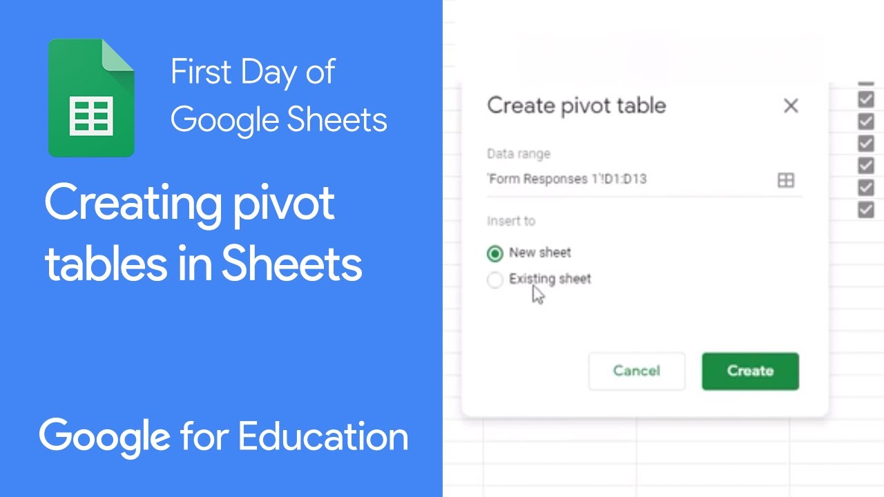
1 Open Google Sheets and locate the spreadsheet that contains the data you want to analyze. Select Data and then Pivot tables from the menu. Then select whether you want to insert the pivot table within the existing sheet or a new sheet.

Now you have a Report Editor window located to the right. Choose where you would want to insert your Pivot Table report in a new sheet or existing sheet. Google Sheets Pivot Tables - Basic Tutorial - YouTube.

A new spreadsheet called Pivot Table opens. Steps to Create a Basic Pivot Table First select the data range A3E8. Highlight the columns that contain your data by clicking and dragging on the headers.

From the Data menu select Pivot Table. If youre going to use everything in your dataset you can click anywhere on the spreadsheet you dont have to select every cell first. Navigate to the Google Sheets Menu select Data and click Pivot Table.

How to Create a Pivot Table. For this guide I will choose the range A1C11. Fire up Chrome and open a spreadsheet in Google Sheets.

This feature allows the user to quickly summarize a large amount of structured data through few clicks giving the user a powerful tool for free. Click Rows in the Pivot table editor and add Property Type clicks three and four 5. Go to Data in the menu bar and select Pivot table.

This will open the Create Pivot Table toolbar. On the right-hand side you see the pivot table editor. For a better overview we will add the table to a new sheet.

Create pivot tables in Google Sheets Select all the data including the headers by selecting the bottom- right corner cell and pressing Ctrl A. Its usually better to. 2 Select the cells with the data you want to use.

Insert a Pivot Table in Google Sheets. Clicks one and two This will create a new tab in your Sheet called Pivot Table 1 or 2 3 4 etc. Now weve prepared our sheet with raw data.

Then click Pivot Table that is under the Data menu. Then go to the upper menu and select Data Pivot Table. The Pivot Table is Google Sheets answer to Microsoft Excels PivotTable feature.

Pivot Table can be a bit more challenging to tame but this tutorial will help you master it by considering the. After that a new sheet will pop up. First open the sheet that contains your data you will use to create a Pivot Table report in Google Sheets and select the data range.

3 Click on Data and in the drop-down menu select Pivot Table. You will be asked if you want to insert your Pivot Table in a new sheet or into your existing sheet. Once youve decided the only thing left to do is to customize the contents and the appearance of your pivot table.

Create your pivot table using your. Click Values in the Pivot table editor and add. Google spreadsheet will ask if you want to create a pivot table in a new sheet or insert it to any existing one.

Right now the Theme is labeled with the box New indicating that it is a recently-added feature in Google Sheets. Next select any of the cells you want to use in your pivot table. Go ahead and highlight the columns where the data is stored and go to the Data Pivot Table option to insert your Pivot table.

Query A1C13 select A sumC group by A pivot B In this example we choose column A to represent the rows of the pivot table column B to represent the columns of the pivot table and the values in column C to be displayed inside the pivot table. Original Pivot Table using Google Sheets Standard theme. Add your desired row and value data.

Creating a new Sheet will name the newly created tab Pivot Table 1 or Pivot Table 2 Pivot Table 3 and so on as you add more. You can use the following syntax to create a pivot table using Google Sheets Query. Open a newly created list with your pivot table.

In Sheets open an existing pivot table or create a new one. As you create more with the Pivot Table framework in place. Open an existing spreadsheet in Google Sheets Select Data from the top menu then Pivot table from the dropdown.

Insert the pivot table.